Note
Click here to download the full example code
Comparison against literature
This example is a comparison of PyHank against results from the original publication of the method.
import numpy as np
import matplotlib.pyplot as plt
import scipy.special as scipybessel

from pyhank import HankelTransform
First we will reproduce figure 1 of
| [1] | “Computation of quasi-discrete Hankel transforms of the integer order for propagating optical wave fields” Manuel Guizar-Sicairos and Julio C. Guitierrez-Vega J. Opt. Soc. Am. A 21 (1) 53-58 (2004) |
First define python functions to calculate the sinc function and its transform
def sinc(x):
    return np.sin(x) / x
Equation 12 of Guizar-Sicairos & Guitierrez-Vega
def hankel_transform_of_sinc(v):
    ht = np.zeros_like(v)
    ht[v < gamma] = (v[v < gamma] ** p * np.cos(p * np.pi / 2)
                     / (2 * np.pi * gamma * np.sqrt(gamma ** 2 - v[v < gamma] ** 2)
                        * (gamma + np.sqrt(gamma ** 2 - v[v < gamma] ** 2)) ** p))
    ht[v >= gamma] = (np.sin(p * np.arcsin(gamma / v[v >= gamma]))
                      / (2 * np.pi * gamma * np.sqrt(v[v >= gamma] ** 2 - gamma ** 2)))
    return ht
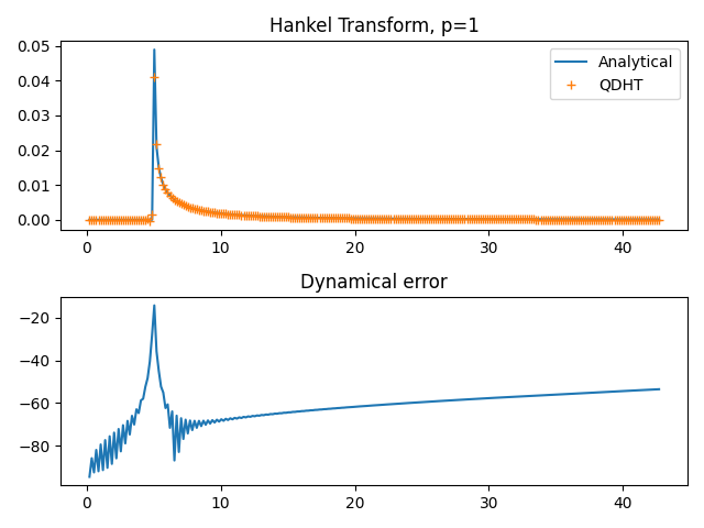
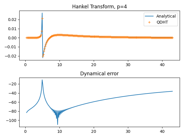
Now plot the values of the hankel transform and the dynamical error as in figure 1 of Guizar-Sicairos & Guitierrez-Vega Guizar for order 1 and 4
for p in [1, 4]:
    transformer = HankelTransform(p, max_radius=3, n_points=256)
    gamma = 5
    func = sinc(2 * np.pi * gamma * transformer.r)
    expected_ht = hankel_transform_of_sinc(transformer.v)
    ht = transformer.qdht(func)
    dynamical_error = 20 * np.log10(np.abs(expected_ht - ht) / np.max(ht))
    not_near_gamma = np.logical_or(transformer.v > gamma * 1.25,
                                   transformer.v < gamma * 0.75)

    plt.figure()
    plt.subplot(2, 1, 1)
    plt.plot(transformer.v, expected_ht, label='Analytical')
    plt.plot(transformer.v, ht, marker='+', linestyle='None', label='QDHT')
    plt.title(f'Hankel Transform, p={p}')
    plt.legend()

    plt.subplot(2, 1, 2)
    plt.plot(transformer.v, dynamical_error)
    plt.title('Dynamical error')
    plt.tight_layout()

    # Check that the error is low, as they do in the paper. Numbers are estimated from their
    # graphs as they do not quote any for this part
    assert np.all(dynamical_error < -10)
    assert np.all(dynamical_error[not_near_gamma] < -35)
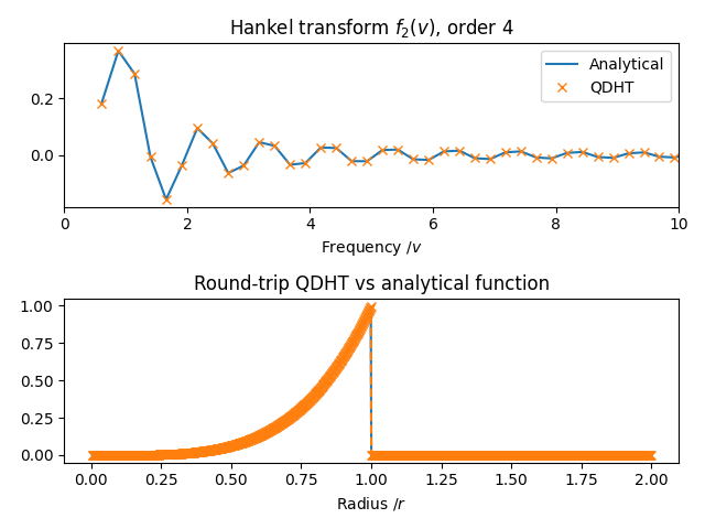
Now we will reproduce figure 3 and confirm we can replicate the errors in the top half of table 1.
p = 4
a = 1
transformer = HankelTransform(order=p, max_radius=2, n_points=1024)
top_hat = np.zeros_like(transformer.r)
top_hat[transformer.r <= a] = 1
func = transformer.r ** p * top_hat
expected_ht = a ** (p + 1) * scipybessel.jv(p + 1, 2 * np.pi * a * transformer.v) / transformer.v
ht = transformer.qdht(func)

retrieved_func = transformer.iqdht(ht)
Plot the overlay as in figure 3 of Guizar-Sicairos & Guitierrez-Vega Guizar
plt.figure()
plt.subplot(2, 1, 1)
plt.plot(transformer.v, expected_ht, label='Analytical')
plt.plot(transformer.v, ht, marker='x', linestyle='None', label='QDHT')
plt.title(f'Hankel transform $f_2(v)$, order {p}')
plt.xlabel('Frequency /$v$')
plt.xlim([0, 10])
plt.legend()

plt.subplot(2, 1, 2)
plt.title('Round-trip QDHT vs analytical function')
plt.plot(transformer.r, func, label='Analytical')
plt.plot(transformer.r, retrieved_func, marker='x', linestyle='--', label='QDHT+iQDHT')
plt.xlabel('Radius /$r$')
plt.tight_layout()
Now check that the error is the same as that given in Table 1 of Guizar-Sicairos & Guitierrez-Vega Guizar
# First calculate e_1 and e_2
error_2 = np.mean(np.abs(expected_ht-ht))
error_1 = np.mean(np.abs(func-retrieved_func))
print(f'Error in Hankel transform is {error_2:.2e}')
print(f'Error in reconstructed function is {error_1:.2e}')
# Note we used 1024 points first
assert np.isclose(error_2, 4.8e-5, atol=1e-6)
# Note that Guizar-Sicairos & Guitierrez-Vega got 2.7e-14, so ours is slightly lower
assert np.isclose(error_1, 2.15e-14, atol=1e-15)
Out:
Error in Hankel transform is 4.81e-05
Error in reconstructed function is 2.15e-14
Now repeat for 512 points
transformer = HankelTransform(order=p, max_radius=2, n_points=512)
top_hat = np.zeros_like(transformer.r)
top_hat[transformer.r <= a] = 1
func = transformer.r ** p * top_hat
expected_ht = a ** (p + 1) * scipybessel.jv(p + 1, 2 * np.pi * a * transformer.v) / transformer.v
ht = transformer.qdht(func)

retrieved_func = transformer.iqdht(ht)

error_2 = np.mean(np.abs(expected_ht-ht))
error_1 = np.mean(np.abs(func-retrieved_func))
print(f'Error in Hankel transform is {error_2:.2e}')
print(f'Error in reconstructed function is {error_1:.2e}')
# Note the below is 10 times smaller than
# #uizar-Sicairos & Guitierrez-Vega (1.3e-3)
assert np.isclose(error_2, 1.3e-4, atol=1e-5)
assert np.isclose(error_1, 2.2e-13, atol=1e-14)
Out:
Error in Hankel transform is 1.35e-04
Error in reconstructed function is 2.25e-13
Total running time of the script: ( 0 minutes 1.377 seconds)