Demonstration of Hankel transform identities

Below we demonstrate a range of known Hankel transform pairs from various sources.

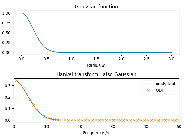
First we demonstrate the Gaussian function from Pissens [1] and its inverse transform.

Then we check the “generalised top-hat” and “generalised jinc” functions from Guizar-Sicairos and Guitierrez-Vega [2].

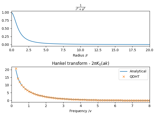
Finally, we look at the function \(f(r) = \frac{1}{r^2 + a^2}\), the Hankel transform of which is \(K_0(av)\), where \(K_0\) is the modified Bessel function of the second kind of order 0. [1]

[1]	(1, 2, 3) “Chapter 9: The Hankel Transform.” Piessens, R. in The Transforms and Applications Handbook: Second Edition. Ed. Alexander D. Poularikas Boca Raton: CRC Press LLC, 2000

[2]	(1, 2, 3) “Computation of quasi-discrete Hankel transforms of the integer order for propagating optical wave fields” Manuel Guizar-Sicairos and Julio C. Guitierrez-Vega J. Opt. Soc. Am. A 21 (1) 53-58 (2004)

import numpy as np
import scipy.special as scipy_bessel
import matplotlib.pyplot as plt

from pyhank import qdht, iqdht, HankelTransform

First we try a Gaussian function, the Hankel transform of which should also be Gaussian.

Note the definition in Guizar-Sicairos [2] varies from that used by Pissens [1] by a factor of \(2\pi\) in both scaling of the argument (so we use HankelTransform.kr rather than HankelTransform.v) and also scaling of the magnitude.

a = 3
radius = np.linspace(0, 3, 1024)
f = np.exp(-a ** 2 * radius ** 2)
kr, actual_ht = qdht(radius, f)
expected_ht = 2*np.pi*(1 / (2 * a**2)) * np.exp(-kr**2 / (4 * a**2))
assert np.allclose(expected_ht, actual_ht)

plt.figure()
plt.subplot(2, 1, 1)
plt.title('Gaussian function')
plt.plot(radius, f)
plt.xlabel('Radius /$r$')
plt.subplot(2, 1, 2)
plt.plot(kr, expected_ht, label='Analytical')
plt.plot(kr, actual_ht, marker='x', linestyle='None', label='QDHT')
plt.title('Hankel transform - also Gaussian')
plt.xlabel('Frequency /$v$')
plt.xlim([0, 50])
plt.legend()
plt.tight_layout()

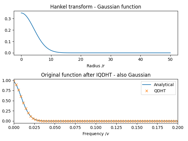
Now we repeat for the inverse transform

kr = np.linspace(0, 50, 1024)
ht = 2*np.pi*(1 / (2 * a**2)) * np.exp(-kr**2 / (4 * a**2))
r, actual_f = iqdht(kr, ht)
expected_f = np.exp(-a ** 2 * r ** 2)
assert np.allclose(expected_f, actual_f)
plt.figure()
plt.subplot(2, 1, 1)
plt.title('Hankel transform - Gaussian function')
plt.plot(kr, ht)
plt.xlabel('Radius /$r$')
plt.subplot(2, 1, 2)
plt.plot(radius, expected_f, label='Analytical')
plt.plot(radius, actual_f, marker='x', linestyle='None', label='QDHT')
plt.title('Original function after IQDHT - also Gaussian')
plt.xlabel('Frequency /$v$')
plt.xlim([0, 0.2])
plt.legend()
plt.tight_layout()

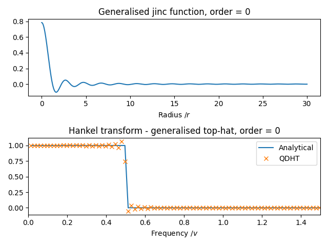
Next we define functions to calculate the generalised top-hat and jinc functions, as defined by Guizar-Sicairos and Guitierrez-Vega [2].

Note that for \(p=0\) these become a standard top-hat and \(\textrm{jinc}(r) = \frac{J_1(r)}{r}\) functions.

def generalised_top_hat(r: np.ndarray, a: float, p: int) -> np.ndarray:
    top_hat = np.zeros_like(r)
    top_hat[r <= a] = 1
    return r ** p * top_hat


def generalised_jinc(v: np.ndarray, a: float, p: int):
    val = np.zeros_like(v)
    val[v != 0] = a ** (p + 1) * scipy_bessel.jv(p + 1, 2 * np.pi * a * v[v != 0]) / v[v != 0]
    if p == -1:
        val[v == 0] = np.inf
    elif p == -2:
        val[v == 0] = -np.pi
    elif p == 0:
        val[v == 0] = np.pi * a ** 2
    else:
        val[v == 0] = 0
    return val

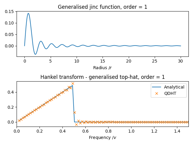
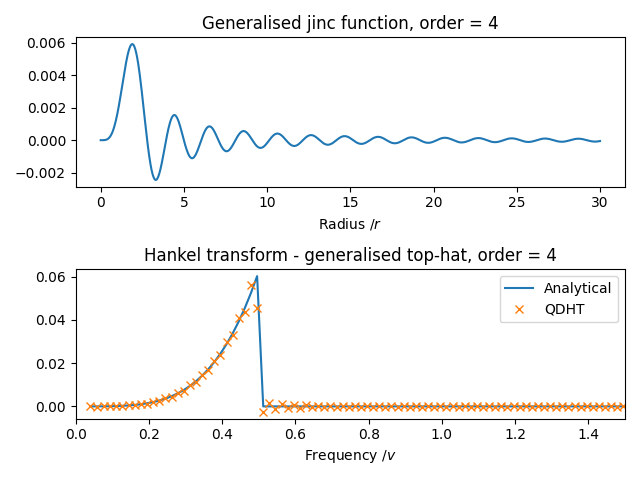
For demonstration, we choose \(a = 0.5\) and run the code for orders 0, 1 and 4 plotting and checking the mean absolute error each time. First check that the Hankel transform of the generalised jinc is calculated correctly.

radius = np.linspace(0, 30, 1024)
a = 0.5
for order in [0, 1, 4]:
    f = generalised_jinc(radius, a, order)
    kr, actual_ht = qdht(radius, f, order=order)
    v = kr / (2*np.pi)
    expected_ht = generalised_top_hat(v, a, order)

    plt.figure()
    plt.subplot(2, 1, 1)
    plt.title(f'Generalised jinc function, order = {order}')
    plt.plot(radius, f)
    plt.xlabel('Radius /$r$')
    plt.subplot(2, 1, 2)
    plt.plot(v, expected_ht, label='Analytical')
    plt.plot(v, actual_ht, marker='x', linestyle='None', label='QDHT')
    plt.title(f'Hankel transform - generalised top-hat, order = {order}')
    plt.xlabel('Frequency /$v$')
    plt.xlim([0, 1.5])
    plt.legend()
    plt.tight_layout()

    error = np.mean(np.abs(expected_ht-actual_ht))
    assert error < 1e-3

• 
• 
• 

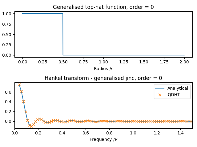
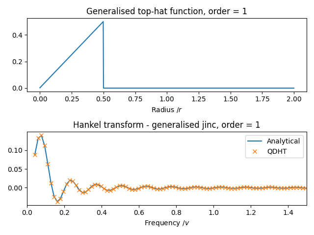
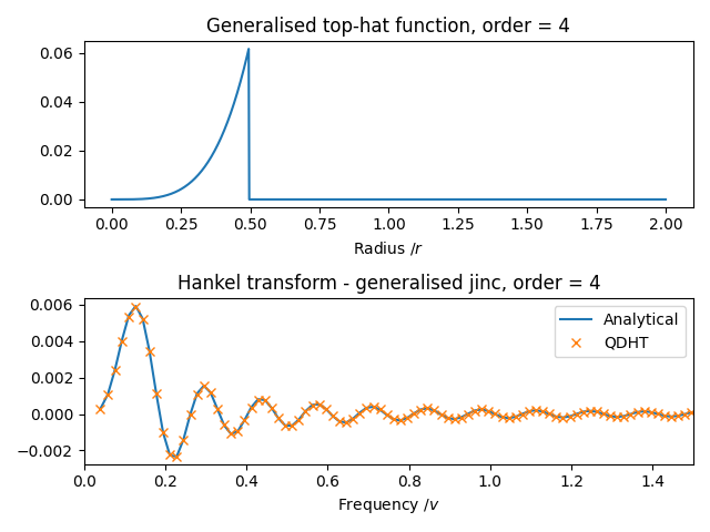
Now we repeat but the other way round: the Hankel transform of the top-hat function should be the jinc function.

radius = np.linspace(0, 2, 1024)
for order in [0, 1, 4]:
    transformer = HankelTransform(order=order, radial_grid=radius)
    f = generalised_top_hat(transformer.r, a, order)
    actual_ht = transformer.qdht(f)
    expected_ht = generalised_jinc(transformer.v, a, order)

    plt.figure()
    plt.subplot(2, 1, 1)
    plt.title(f'Generalised top-hat function, order = {order}')
    plt.plot(radius, f)
    plt.xlabel('Radius /$r$')
    plt.subplot(2, 1, 2)
    plt.plot(v, expected_ht, label='Analytical')
    plt.plot(v, actual_ht, marker='x', linestyle='None', label='QDHT')
    plt.title(f'Hankel transform - generalised jinc, order = {order}')
    plt.xlabel('Frequency /$v$')
    plt.xlim([0, 1.5])
    plt.legend()
    plt.tight_layout()

    error = np.mean(np.abs(expected_ht - actual_ht))
    assert error < 1e-3

• 
• 
• 

Now we investigate the function \(f(r) = \\frac{1}{r^2 + a^2}\), the Hankel transform of which is \(K_0(av)\).

Note again the scaling factor of \(2\pi\).

a = 1
radius = np.linspace(0, 50, 1024)
transformer = HankelTransform(order=0, radial_grid=radius)
f = 1 / (transformer.r**2 + a**2)
actual_ht = transformer.qdht(f)
expected_ht = 2 * np.pi * scipy_bessel.kn(0, a * transformer.kr)

plt.figure()
plt.subplot(2, 1, 1)
plt.title('$\\frac{1}{r^2 + a^2}$')
plt.plot(radius, f)
plt.xlabel('Radius /$r$')
plt.xlim([0, 20])

plt.subplot(2, 1, 2)
plt.plot(kr, expected_ht, label='Analytical')
plt.plot(kr, actual_ht, marker='x', linestyle='None', label='QDHT')
plt.title(r'Hankel transform - $2 \pi K_0(ak)$')
plt.xlabel('Frequency /$v$')
plt.xlim([0, 8])
plt.legend()
plt.tight_layout()