Typical usage

To demonstrate the use of the Hankel Transform class, we will give an example of propagating a radially-symmetric beam using the beam propagation method.

In this case, it will be a simple Gaussian beam propagating way from focus and diverging.

First we will use a loop over \(z\) position, and then we will demonstrate the vectorisation of the HankelTransforms.iqdht() (and qdht()) functions.

First import the standard libraries

import matplotlib.pyplot as plt
import numpy as np

Then the functions from this package

from pyhank import HankelTransform
# noinspection PyUnresolvedReferences
from helper import gauss1d, imagesc

Initialise radius grid

nr = 1024  # Number of sample points
r_max = 5e-3  # Maximum radius (5mm)
r = np.linspace(0, r_max, nr)

Initialise \(z\) grid

Nz = 200  # Number of z positions
z_max = 0.1  # Maximum propagation distance
z = np.linspace(0, z_max, Nz)  # Propagation axis

Set up beam parameters

Dr = 100e-6  # Beam radius (100um)
lambda_ = 488e-9  # wavelength 488nm
k0 = 2 * np.pi / lambda_  # Vacuum k vector

Set up a HankelTransform object, telling it the order (0) and the radial grid.

H = HankelTransform(order=0, radial_grid=r)

Set up the electric field profile at \(z = 0\), and resample onto the correct radial grid (transformer.r) as required for the QDHT.

Er = gauss1d(r, 0, Dr)   # Initial field
ErH = H.to_transform_r(Er)  # Resampled field

Perform Hankel Transform

# Convert from physical field to physical wavevector
EkrH = H.qdht(ErH)

Propagate the beam - loop

Do the propagation in a loop over \(z\)

# Pre-allocate an array for field as a function of r and z
Erz = np.zeros((nr, Nz), dtype=complex)
kz = np.sqrt(k0 ** 2 - H.kr ** 2)
for i, z_loop in enumerate(z):
    phi_z = kz * z_loop  # Propagation phase
    EkrHz = EkrH * np.exp(1j * phi_z)  # Apply propagation
    ErHz = H.iqdht(EkrHz)  # iQDHT
    Erz[:, i] = H.to_original_r(ErHz)  # Interpolate output
Irz = np.abs(Erz) ** 2

Plotting

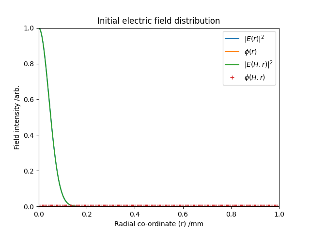
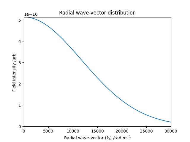
Plot the initial field and radial wavevector distribution (given by the Hankel transform)

plt.figure()
plt.plot(r * 1e3, np.abs(Er) ** 2, r * 1e3, np.unwrap(np.angle(Er)),
         H.r * 1e3, np.abs(ErH) ** 2, H.r * 1e3, np.unwrap(np.angle(ErH)), '+')
plt.title('Initial electric field distribution')
plt.xlabel('Radial co-ordinate (r) /mm')
plt.ylabel('Field intensity /arb.')
plt.legend(['$|E(r)|^2$', '$\\phi(r)$', '$|E(H.r)|^2$', '$\\phi(H.r)$'])
plt.axis([0, 1, 0, 1])

plt.figure()
plt.plot(H.kr, np.abs(EkrH) ** 2)
plt.title('Radial wave-vector distribution')
plt.xlabel(r'Radial wave-vector ($k_r$) /rad $m^{-1}$')
plt.ylabel('Field intensity /arb.')
plt.axis([0, 3e4, 0, np.max(np.abs(EkrH) ** 2)])

• 
• 

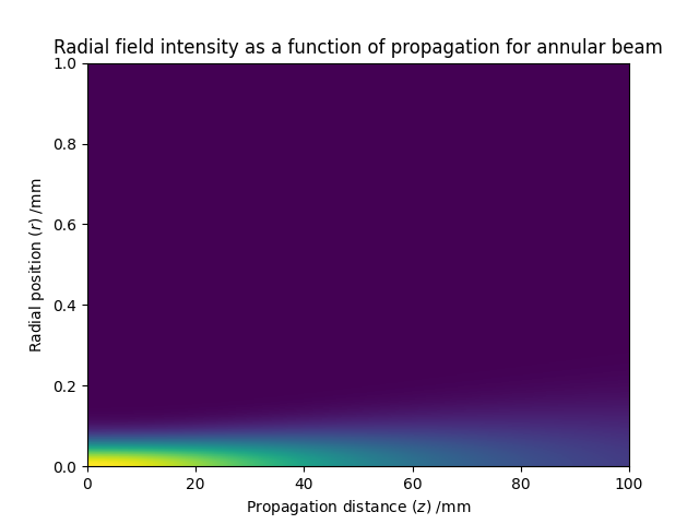
Now plot an image showing the intensity as a function of radius and propagation distance.

plt.figure()
imagesc(z * 1e3, r * 1e3, Irz)
plt.title('Radial field intensity as a function of propagation for annular beam')
plt.xlabel('Propagation distance ($z$) /mm')
plt.ylabel('Radial position ($r$) /mm')
plt.ylim([0, 1])

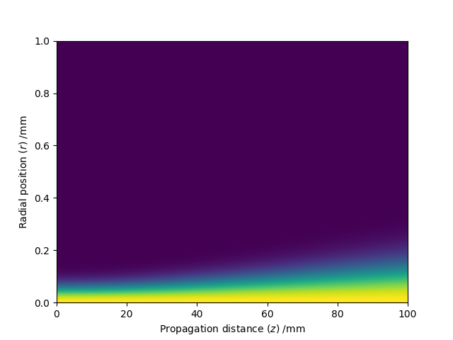
The plot above shows a reduction of intensity with \(z\), but it is bit difficult to see the beam growing in \(r\). To show that, let’s plot the intensity normalised such that the peak intensity at each \(z\) coordinate is the same.

Irz_norm = Irz / Irz[0, :]

plt.figure()
imagesc(z * 1e3, r * 1e3, Irz_norm)
plt.xlabel('Propagation distance ($z$) /mm')
plt.ylabel('Radial position ($r$) /mm')
plt.ylim([0, 1])

Propagate the beam - vectorised

kz = np.sqrt(k0 ** 2 - H.kr ** 2)
phi_z = kz[:, np.newaxis] * z[np.newaxis, :]  # Propagation phase
EkrHz = EkrH[:, np.newaxis] * np.exp(1j * phi_z)  # Apply propagation
ErHz = H.iqdht(EkrHz)  # iQDHT
Erz = H.to_original_r(ErHz)  # Interpolate output
Irz_vectorised = np.abs(Erz) ** 2

Now plot the result to check it is the same as the loop approach

plt.figure()
imagesc(z * 1e3, r * 1e3, Irz_vectorised)
plt.title('Radial field intensity as a function of propagation for annular beam')
plt.xlabel('Propagation distance ($z$) /mm')
plt.ylabel('Radial position ($r$) /mm')
plt.ylim([0, 1])

Assert the two approaches produce the same intensity

assert np.allclose(Irz, Irz_vectorised)