Speed of single-shot vs reuse of a HankelTransform object

For a simple case (as in Example of single-shot transform) there are two simple forward qdht() and [inverse iqdht()] functions which can be used to calculate the [inverse] Hankel transform of a function sampled at an arbitrary set of points in radius [wave-number] space.

Here we will use the same example application as Typical usage: a beam-propagation method propagation of a radially-symmetric Gaussian beam.

import time

import numpy as np
from scipy import interpolate
import matplotlib.pyplot as plt

from pyhank import HankelTransform, qdht, iqdht
from helper import gauss1d, imagesc

Initialise radius and \(z\) grids and beam parameters as in Typical usage.

nr = 1024  # Number of sample points
r_max = 5e-3  # Maximum radius (5mm)
Nz = 100  # Number of z positions
z_max = 0.1  # Maximum propagation distance

r = np.linspace(0, r_max, nr)
z = np.linspace(0, z_max, Nz)

Dr = 100e-6  # Beam radius (100um)
lambda_ = 488e-9  # wavelength 488nm
k0 = 2 * np.pi / lambda_  # Vacuum k vector

field = gauss1d(r, 0, Dr)   # Initial field

Now we need two functions that propagate the beam in two ways (giving the same answer). The first will use single shot, the second will use a HankelTransform object. Below we will run each of them in turn and compare the speed.

def propagate_using_object(r: np.ndarray, field: np.ndarray) -> np.ndarray:
    transformer = HankelTransform(order=0, radial_grid=r)
    field_for_transform = transformer.to_transform_r(field)  # Resampled field
    hankel_transform = transformer.qdht(field_for_transform)

    propagated_field = np.zeros((nr, Nz), dtype=complex)
    kz = np.sqrt(k0 ** 2 - transformer.kr ** 2)
    for n, z_loop in enumerate(z):
        phi_z = kz * z_loop  # Propagation phase
        hankel_transform_at_z = hankel_transform * np.exp(1j * phi_z)  # Apply propagation
        field_at_z_transform_grid = transformer.iqdht(hankel_transform_at_z)  # iQDHT
        propagated_field[:, n] = transformer.to_original_r(field_at_z_transform_grid)  # Interpolate output
    intensity = np.abs(propagated_field) ** 2
    return intensity


def propagate_using_single_shot(r: np.ndarray, field: np.ndarray) -> np.ndarray:
    kr, hankel_transform = qdht(r, field)

    propagated_field = np.zeros((nr, Nz), dtype=complex)
    kz = np.sqrt(k0 ** 2 - kr ** 2)
    for n, z_loop in enumerate(z):
        phi_z = kz * z_loop  # Propagation phase
        hankel_transform_at_z = hankel_transform * np.exp(1j * phi_z)  # Apply propagation
        r_transform, field_at_z_transform_grid = iqdht(kr, hankel_transform_at_z)  # iQDHT
        f = interpolate.interp1d(r_transform, field_at_z_transform_grid, axis=0,
                                 fill_value='extrapolate', kind='cubic')
        propagated_field[:, n] = f(r)
    intensity = np.abs(propagated_field) ** 2
    return intensity

Now run and time the two functions:

tic = time.time()
single_shot_intensity = propagate_using_single_shot(r, field)
toc = time.time()
print(f'Single shot propagation took {toc-tic:.2f} s')

tic = time.time()
object_intensity = propagate_using_object(r, field)
toc = time.time()
print(f'Object propagation took {toc-tic:.2f} s')

Out:

Single shot propagation took 51.73 s
Object propagation took 0.93 s

The single shot approach takes a lot longer!

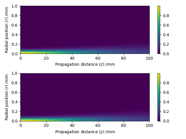
Plot the two results to check they are the same:

plt.figure()
plt.subplot(2, 1, 1)
imagesc(z * 1e3, r * 1e3, single_shot_intensity)
plt.xlabel('Propagation distance ($z$) /mm')
plt.ylabel('Radial position ($r$) /mm')
plt.colorbar()
plt.ylim([0, 1])

plt.subplot(2, 1, 2)
imagesc(z * 1e3, r * 1e3, object_intensity)
plt.xlabel('Propagation distance ($z$) /mm')
plt.ylabel('Radial position ($r$) /mm')
plt.ylim([0, 1])
plt.colorbar()
plt.tight_layout()